|
时间趋势图可以粗略地对政策实施前后处理组与对照组样本之间的变化趋势做出判断,是进行DID研究的前提所在。 graph set window fontface "Times New Roman"graph set window fontfacesans "宋体" // 设置图形输出的字体 egen mean_y=mean(entre_activation), by(year group) graph twoway (connect mean_y year if group==1,sort) (connect mean_y year if group==0,sort lpattern(dash)), /// xline(2010,lpattern(dash) lcolor(gray)) /// ytitle("{stSans:创}""{stSans:业}""{stSans:活}""{stSans:跃}""{stSans:度}",orientation(h)) xtitle("{stSans:年度}") /// ylabel(0(0.5)3,labsize(*0.75) format(%02.1f)) xlabel(,labsize(*0.75)) /// legend(label(1 "{stSans:处理组}") label( 2 "{stSans:控制组}")) ///图例 xlabel(2004 (1) 2018) graphregion(color(white)) //白底 graph export "平行趋势事前检验.png"
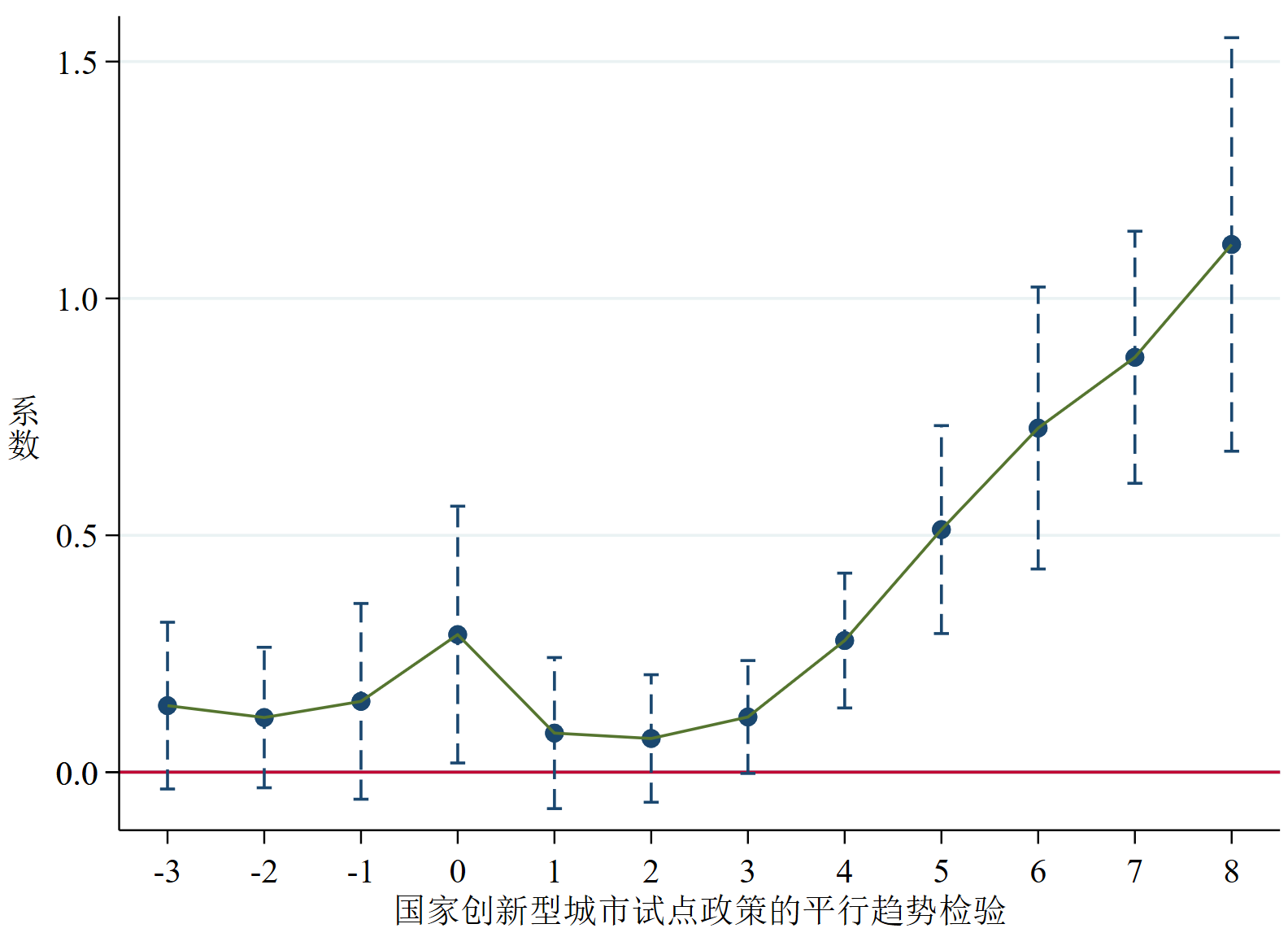
如图 1 所示,以 2010 年国家创新型城市试点为例,2010 年之后,试点城市(处理组)的创业活跃度相对于非试点城市(对照组)经历了更高程度的增长,二者的创业活跃度差距逐渐扩大,而在 2010 年之前,二者具有较为一致的变化趋势。 5.2 事件分析法事件分析法检验平行趋势最常见的一种方法,一般模型构造如下: $$\operatorname Y_{i ,t}=\beta_{0}+\sum_{-k}^{s} \beta_{m} D_{i, t}^{m}+\gamma X_{i ,t}+\mu_{i}+\lambda _t+\varepsilon_{i, t} $$ 时间虚拟变量 D_{i,t}^{m} 表示各城市确立为试点城市前 k 年、当年和后 s 年的观测值,非试点城市虚拟变量均为 0。白俊红等(2022)中,考虑到政策实施时间与试点数量等因素,取 k=3,s=8。本推文提供以下三种检验方法,详细经济学含义请参考原文。 (1)手动计算各时期虚拟变量,coefplot辅助作图(1)代码一 xtset city yeargen event = year - branch_reform if group==1 replace event = -4 if event <= -4 tab event, gen(eventt) forvalues i = 1/15{ replace eventt`i' = 0 if eventt`i' == . } drop eventt1 xtreg entre_activation eventt* $xlist i.year, r fe (2)代码二 gen distance=year-ptreplace distance = -4 if distance <= -4 tab distance,missing forvalues i=1/4{ gen d_`i' = 0 replace d_`i' = 1 if Treat== 1 & distance== -`i' } forvalues i=1/10 { gen d`i' = 0 replace d`i' = 1 if Treat== 1 & distance== `i' } gen d0 = 0 replace d0 = 1 if Treat== 1 & distance== 0 xtset city year xtreg entre_activation d_3 d_2 d_1 d0 d1-d10 $xlist i.year,fe r graph export "平行趋势检验.png",as(png) replace width(800) height(600) 上述两种方法对于时间虚拟变量的计算结果完全相同,不同之处在于代码一在运用coefplot绘图时需要将eventt*转换为基于政策前后的数值,代码二则可以直接绘图,平行趋势图如下:
据上图所知,政策发生前的相对时间虚拟变量系数均不显著且数值较小,表明政策发生之前,处理组与对照组在创业活跃度上无显著差异,满足平行趋势假设。进一步从动态效应来看,在政策发生后当年,试点政策短暂产生创业效应但还未稳定,试点政策推行 3 年后,创新型城市试点政策的影响系数显著为正并不断提升,表明创新型城市试点政策能够产生促进创业活跃度提升的政策效应,但具有一定的滞后性。 (2)tvdiff命令实现tvdiff能够实现仅运行一条命令就可以同时实现图示处理期前后处理效应,以及呈现平行趋势检验统计结果。可以参考推文Stata:多期倍分法 (DID) 详解及其图示,已对该方法做了详细讲解,也可以直接help tvdiff查询官网教程和数据获取。本推文重点在整理该方法,不再展开。 (3)eventdd命令的Stata操作(1)命令安装 ssc install eventdd, replace //安装命令(2)语法结构 eventdd命令是 Damian Clarke & Kathya Tapia Schythe (2021) 在现有事件分析法的基础上所编写的 Stata 新命令,其语法结构如下: eventdd depvar [indepvars] [ if ] [ in ] [ weight ] , ///timevar(timevar) ci(type, ...) [ method baseline(#) level(#) accum lags(#) leads(#) noend noline keepbal(varname) absorb(varname) wboot wboot_op(string) balanced inrange graph_op(string) ci_op(string) coef_op(string) endpoints_op(string)] depvar:被解释变量; indepvars:控制变量; timevar:必须,设定时间政策变量,与前文 year-policy 相同; ci (type, ...):指定置信区间的图形类型:rarea (带区域阴影)、rcap (带封顶尖钉)、rline (带线条),rcap 是默认的图表类型; method (type, [absorb (absvars)] * ...):指定估计方法,默认为ols,xtreg对应fe,hdfe对应absorb (absvars); baseline (#):指定政策时间相对基准期,默认为 - 1; level (#):设置置信度;默认值为 95%; lags (#):指明事件研究中要考虑的最大事件后时段,在accum、keepbal、inrange指定时,必须确定; `leads (#):指明事件研究中要考虑的最大事件前期数,同上; accum:指定超出某些指定值的所有时期都应累积到最终点数中; noend:当指定 accum 选项时,要求累积终点不显示在图形输出上; keepbal (varname):指定只保留面板中平衡的单位以供估计。这里varname 表示指示单位的面板变量(如 state); balanced:要求只绘制 “平衡的” 提前和滞后期; inrange:要求只绘制指定期数的提前和滞后期图形; noline:删除 - 1 这条基准线; wboot:要求用wild bootstrap估计置信区间; wboot_op (string):指定任意选项用于wild bootstrap估计,(例如seed ()、bootcluster ()); graph_op (string):允许包含twoway中允许的任何其他通用图形选项,包括标题、线型、轴标签等; coef_op (string):允许包含scatter中的图形选项; endpoints_op:允许包含端点系数的scatter图形选项,须在accum下使用; (3)实例教学 下面我们使用作者提供的数据来检验此命令。 webuse setwebuse bacon_example.dta, clear //导入数据 xtset stfips year xtreg asmrs post pcinc asmrh cases i.year, fe cluster(stfips) gen timeToTreat = year - _nfd //设定时间政策变量 作者使用了 Stevenson 和 Wolfers(2006)关于美国无过错离婚改革和女性自杀的数据。数据包括 49 个州从 1964 年至 1996 年的面板数据,各州单方面离婚改革的时间不同。 eventdd asmrs pcinc asmrh cases i.year, timevar(timeToTreat) method(fe, cluster(stfips)) graph_op(ytitle("Suicidesper 1m Women") xlabel(-20(5)25))graph export "Event Study Example Based on No-fault Divorce Reforms.png", replace eventdd asmrs pcinc asmrh cases i.year, fe timevar(timeToTreat) ci(rcap) inrange leads(10) lags(10) cluster(stfips) graph_op(ytitle("Suicides per 1m Women")) graph export "Show periods between -10 y 10.png", replace eventdd asmrs pcinc asmrh cases i.year, fe timevar(timeToTreat) ci(rcap) balanced cluster(stfips) graph_op(ytitle("Suicides per 1m Women")) graph export "Show balanced periods.png", replace eventdd asmrs pcinc asmrh cases, hdfe timevar(timeToTreat) ci(rcap) cluster(stfips) absorb(i.stfips i.year) keepbal(stfips) leads(10) lags(10) graph_op(ytitle("Suicidesper 1m Women")) graph export "Only balanced units between -10 y 10.png", replace eventdd asmrs pcinc asmrh cases i.year, fe timevar(timeToTreat) ci(rcap) cluster(stfips) accum leads(15) lags(10) graph_op(ytitle("Suicidesper 1m Women")) graph export "Accumulating into end points -15 y 10.png", replace eventdd asmrs pcinc asmrh cases i.year, timevar(timeToTreat) method(fe, cluster(stfips)) accum noend leads(15) lags(10) graph_op(ytitle("Suicidesper 1m Women") ) graph export "Not showing end points.png", replace 上述对应的 6 组代码分别对应下图 a-f 的平行趋势检验情况,表明eventdd命令在运用事件分析法检验平行趋势时可以灵活处理不同时期,功能十分强大。
graph export "Plot with alternative appearance options.png", replace 下图展示了调整外观之后的平行趋势检验图,可以很直观看出在政策实施前,散点在红线附近波动,表明政策实施前无过错离婚改革和女性自杀具有一致变化趋势。
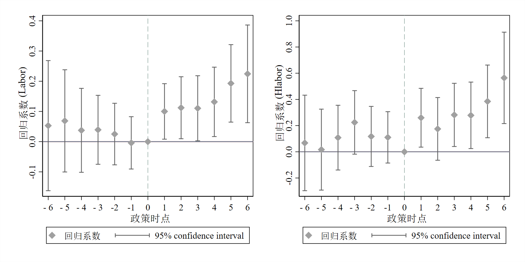
(4)论文应用 余明桂等(2022)在研究专利质押政策对企业劳动雇佣关系时,运用了eventdd命令来识别政策平行趋势。左图表明,在专利质押政策实施前,试点地区与非试点地区的劳动雇佣并不存在显著差异,而政策试点对劳动雇佣的影响出现在政策实施一年及以后。右图显示,专利质押政策出台前,试点地区与非试点地区的高技术水平员工规模并不存在显著差异,在政策实施后,企业高技术员工规模的增长存在一定持续性。 以上结果支持了平行趋势假设。 use 专利质押,clearglobal c "Size Lev Roa Soe p_GDP Second_ind " xtset code year replace Policy_year=. if Policy_year==0 gen yeardif=year-Policy_year eventdd Labor $c i.year, timevar(yeardif) method(fe) cluster(code) level(95) baseline(0) noline /// graph_op( yline(0,lcolor(edkblue*0.8) ) /// xlabel(-6 "- 6" -5 "- 5" -4 "- 4" -3 "- 3" -2 "-2" -1 "-1" 0 "0" 1 "1" 2 "2" 3 "3" 4 "4" 5 "5" 6 "6") /// ylabel(-0.1(0.1)0.4,format (%7.1f)) /// xline(0 ,lwidth(vthin) lpattern(dash) lcolor(teal)) /// xtitle(`"{fontface "宋体": 政策时点}"', size(medium small)) /// ytitle(`"{fontface "宋体": 回归系数}{stSerif: (Labor)}"', size(medium small)) /// legend(order(2 `"{fontface "宋体": 回归系数}"' 1 "95% confidence interval" )) scheme(s1mono)) graph save "平行趋势Labor.gph", replace eventdd Hlabor $c i.year, timevar(yeardif) method(fe) cluster(code) level(95) baseline(0) noline /// graph_op( yline(0,lcolor(edkblue*0.8) ) /// xlabel(-6 "- 6" -5 "- 5" -4 "- 4" -3 "- 3" -2 "-2" -1 "-1" 0 "0" 1 "1" 2 "2" 3 "3" 4 "4" 5 "5" 6 "6") /// ylabel(-0.2(0.2)1,format (%7.1f)) /// xline(0 ,lwidth(vthin) lpattern(dash) lcolor(teal)) /// xtitle(`"{fontface "宋体": 政策时点}"', size(medium small)) /// ytitle(`"{fontface "宋体": 回归系数}{stSerif: (Hlabor)}"', size(medium small)) /// legend(order(2 `"{fontface "宋体": 回归系数}"' 1 "95% confidence interval" )) scheme(s1mono)) graph save "平行趋势Hlabor.gph", replace graph combine 平行趋势Labor.gph 平行趋势Hlabor.gph,col(2) row(1) iscale(1) xsize(10) ysize(5)
|